Study 2
Evaluating scaffolds for an unconventional statistical graph
Introduction
In Study Two we examine if scaffolding is effective in aiding
untrained students to understand the Triangular Model (TM) graph. We
know that students are unlikely to construct the correct interpretation
of the TM without assistance. Guided by the results of the Study One
Design Task, we created four scaffolds. We test the effectiveness of
these scaffolds by seeking to replicate the Qiang et.al (2014) finding
that after 20 minutes of video training, students perform faster and
more accurately with the unconventional TM than the conventional Linear
Model (LM). Will our participants show similar performance on the TM
with scaffolds rather than formal instruction? Further, will engagement
with the TM in a reading task be sufficient for students to reproduce
the graph in a subsequent drawing task?
Hypotheses
- Learners without scaffolding (control) will perform better with the
LM than TM
- Learners with (any form of) scaffolding will perform better with the
TM than LM (replication of [12]).
- Based on observations in Study One we expect that graph-order will
act as a scaffold. Learners who solve problems with the LM graph first
will perform better on the TM (relative to TM-first learners) as their
attention will be drawn to the salient differences between the
graphs.
To try the study yourself: visit http://morning-gorge-17056.herokuapp.com/
Enter “github” as your session code, and number of the condition you
wish to test
0 = control (no-scaffold), 1 = “what-text”, 2 = “how-text”, 3 =
“static-image”, 4 = “interactive-image”
Methods
Design
We employed a 5 (scaffold: none-control, what-text, how-text, static
image, interactive image) x 2 (graph: LM, TM) mixed design, with
scaffold as a between-subjects variable and graph as a within-subject
variable. To test our hypothesis that exposure to the conventional LM
acts as a scaffold for the TM, we counterbalanced the order of
graph-reading tasks (order: LM-first, TM-first). For each task we
measured response accuracy and time. For the follow-up graph-drawing
task, a team of raters coded the type of graph produced by each
participant.
Participants
316 (69% female) students aged 17 to 33 at a public American
univeristy participated in the study. All participants completed three
activities: two graph reading tasks (with both the linear model (LM) and
triangular model (TM) graphs) followed by a drawing task. In some cases
(linear-first), participants (n = 154) completed the graph reading task
with the LM graph, followed by the task with the TM graph. An additional
(n= 162) subjects completed the graph reading tasks in reverse order.
Each particiant was randomly assigned to one of five conditions which
determined what additional information (scaffold) they received while
solving the first five problems with each graph: no-scaffold (control),
‘what’ text, ‘how’-text, static-image, and interactive-image. The
runtime of the entire study ranged from 22 to 66 minutes (m = 40, sd =
0.48).
Materials
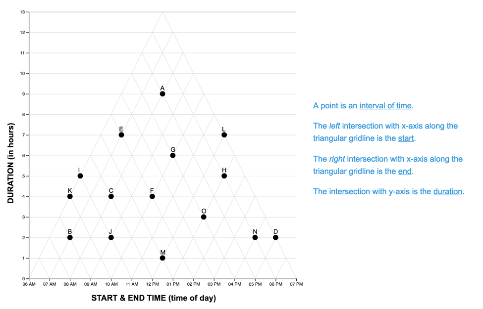
Scaffolds
For the first five questions of each graph-reading task, participants
saw their assigned scaffold along with the designated graph. On the
following ten questions, the scaffold was not present. Examples of each
scaffold-condition for the TM and LM graphs are shown below.
| Scaffold Condition | Linear Model (LM) | Triangular Model (LM) | |
|---|---|---|---|
| none-control | 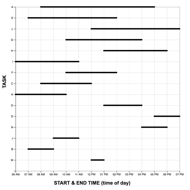 |
 |
|
| "what-text" |  |
 |
|
| "how-text" | 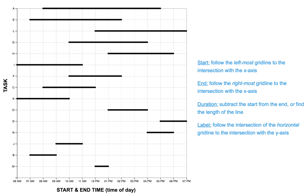 |
 |
|
| "static-image" | 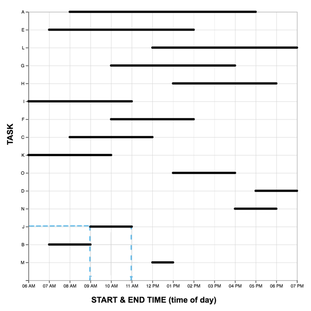 |
 |
|
| "interactive-image" | 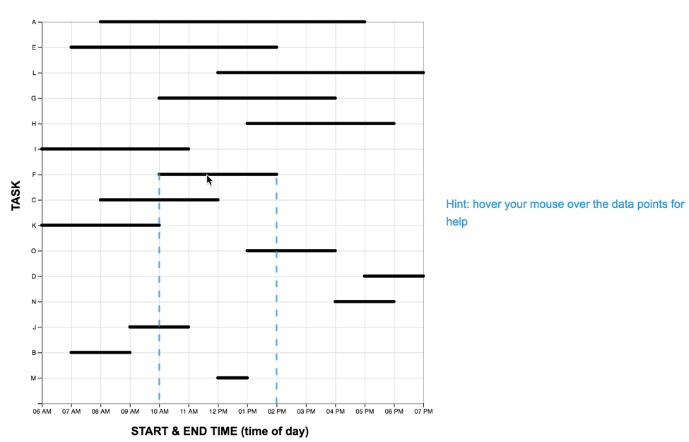 |
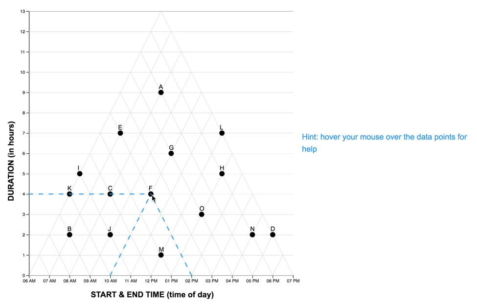 |
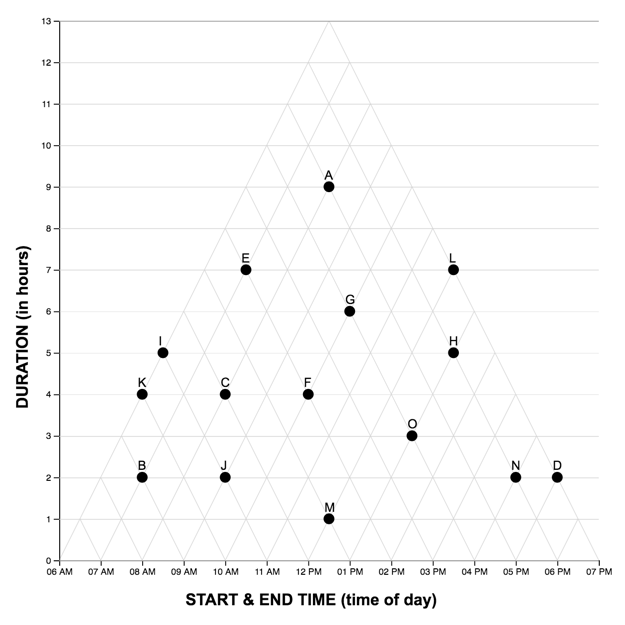
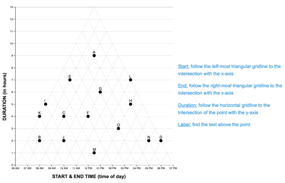
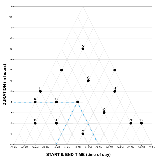
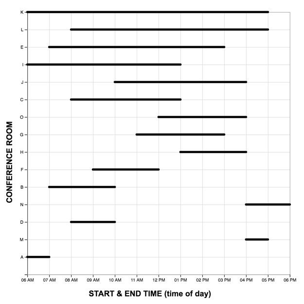
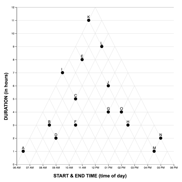
The Graph Reading Task
Each graph reading task consisted of a graph (LM or TM) and 15 multiple choice questions (used in Study One). Questions were presented one at a time, and participants did not receive feedback as to the accuracy of their response before proceeding to the next question. The order of the first five (scaffolded) questions was the same for each participant, while the order of the remaining 10 were randomized. For each question, the stimulus software recorded the participant’s response accuracy (correct, incorrect) and latency (time from page-load to “submit” button press). As each participant completed the reading task once with each graph, we developed two matched scenarios: a project manager scheduling tasks (scenario A), and an events manager scheduling reservations (scenario B). In each scenario, an equivalent question can be identified in the other pertaining to the same interval property or relation. For the LM graphs, intervals were sorted in order of duration, with the longest intervals appearing at the top of the graph.A pilot study on Amazon Mechanical Turk using the LM graph revealed no significant differences in difficulty between the scenarios. The four graphs constructed for the study are shown below.
The full list of questions and correct answers can be found here .
| Task Scheduling (Scenario A) | Event Scheduling (Scenario B) |
|---|---|
 |
 |
|
 |
|
 |
The Graph Drawing Task
In the graph drawing task participants were given a sheet of
isometric dot paper and a table containing a set of 10 time intervals.
Isometric dot paper equally supports the construction of lines at 0, 45
and 90 degrees, thus minimizing any biasing effects of the paper on the
type of graph the participants chose to draw. Participants were directed
to draw a triangular graph of the data (“like the triangle graph you saw
in the previous task”), using the pencil, eraser and ruler provided.
Procedure
Participants completed the study individually in a computer lab.
After a short introduction they continued to the first of two graph
reading tasks (graph order counterbalanced). After completing the first
graph reading task, they were introduced to the second scenario, and
completed the second graph reading task with the remaining graph.
Finally, participants completed the graph drawing task. They finished
the study by completing a short demographic survey, and reading the
debriefing text.
Results (Score)
###Explore the data We see a large variance in TM scores across Graph-Orders
#EXPLORE THE DATA
#create boxplot

#SIMPLE BOXPLOT BY CONDITION
# mixedPlot_condition <- ggplot(l_scores, aes(condition,value, color=variable))+ geom_boxplot() +
#  labs(x="scaffold condition", y="score (max = 15)") +
#  ggtitle("Task Score by Scaffold ") +
#  theme_bw()
# mixedPlot_condition

#BOXPLOT BY CONDITION, FACET WITH ORDER
mixedPlot_order <- ggplot(l_scores, aes(condition,value, fill=variable))+ geom_boxplot() +
  facet_wrap(~order, labeller=labeller(order = order_labels)) +
  labs(x="scaffold condition", y="score (max = 15)", color="task")+
  labs(title="Task Score by Scaffold & Graph-Order ") +
  theme_bw() +
  theme(strip.background = element_blank()) +
  scale_fill_manual( values = c(green,red),
                       name="graphing task",
                       breaks=c("linear_score", "triangular_score"),
                       labels=c("linear", "triangular"))
mixedPlot_order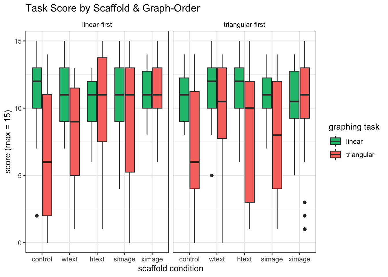
#BOXPLOT BY CONDITION, FACET WITH ORDER AND SCENARIO
mixedPlot_scenario <- ggplot(l_scores, aes(condition,value, fill=variable))+ geom_boxplot() +
 facet_grid(lm_scenarios~order, labeller=labeller(order = order_labels)) +
 labs(x="scaffold condition", y="score (max = 15)")+
 ggtitle("Task Score by Scaffold, Task Order and Scenario ") +
 theme_bw() +
 theme(strip.background = element_blank()) +
 scale_fill_manual( values = c(green,red),
                       name="graphing task",
                       breaks=c("linear_score", "triangular_score"),
                       labels=c("linear", "triangular"))
  #use scale_fill_manual to manually change colors
mixedPlot_scenario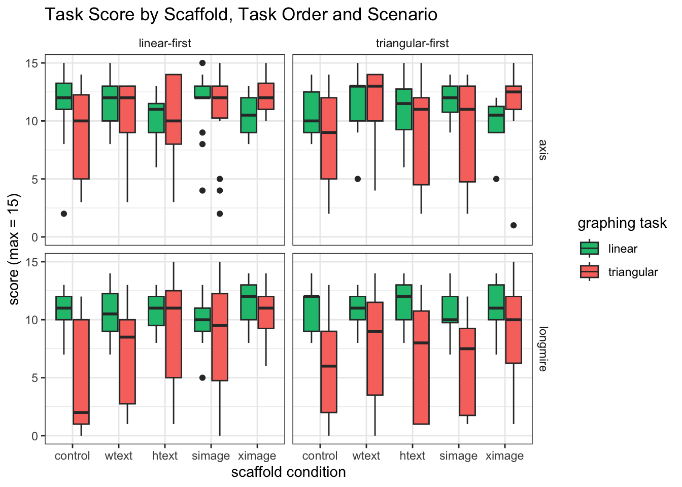
Hypothesis 1: Scaffold conditon and graph-order will not affect performance on the LM graph, because it is conventional and relatively easy to read
When we compare LM scores both graph-orders and scaffold-conditions (and scenarios), we do not find significant differences
#explore descriptive statistics based on each IV

#LM SCORES BY SCAFFOLD
desc_control <- by(w_scores$linear_score, list(w_scores$condition), stat.desc, basic=FALSE)
desc_control
## : 0
##       median         mean      SE.mean CI.mean.0.95          var      std.dev
##   11.0000000   10.9836066    0.2979821    0.5960530    5.4163934    2.3273146
##     coef.var
##    0.2118898
## ------------------------------------------------------------
## : 1
##       median         mean      SE.mean CI.mean.0.95          var      std.dev
##   11.0000000   11.0677966    0.2848856    0.5702604    4.7884278    2.1882477
##     coef.var
##    0.1977130
## ------------------------------------------------------------
## : 2
##       median         mean      SE.mean CI.mean.0.95          var      std.dev
##   11.0000000   10.8939394    0.2618998    0.5230500    4.5270396    2.1276841
##     coef.var
##    0.1953090
## ------------------------------------------------------------
## : 3
##       median         mean      SE.mean CI.mean.0.95          var      std.dev
##   11.0000000   10.9193548    0.2790958    0.5580865    4.8294553    2.1976022
##     coef.var
##    0.2012575
## ------------------------------------------------------------
## : 4
##       median         mean      SE.mean CI.mean.0.95          var      std.dev
##   11.0000000   10.8970588    0.2286922    0.4564716    3.5564091    1.8858444
##     coef.var
##    0.1730599

#LM SCORES BY GRAPH-ORDER
desc_control <- by(w_scores$linear_score, list(w_scores$order), stat.desc, basic=FALSE)
desc_control
## : LMFirst
##       median         mean      SE.mean CI.mean.0.95          var      std.dev
##   11.0000000   10.8636364    0.1767556    0.3491966    4.8113488    2.1934787
##     coef.var
##    0.2019102
## ------------------------------------------------------------
## : TMFirst
##       median         mean      SE.mean CI.mean.0.95          var      std.dev
##   11.0000000   11.0308642    0.1629851    0.3218642    4.3033893    2.0744612
##     coef.var
##    0.1880597

#ONE WAY ANOVA ON LM_SCORE BY SCAFFOLD
#construct contrasts for ANOVA model
options(contrasts=c("contr.sum","contr.poly"))

simpleModel = ezANOVA(data = w_scores,
                     dv = .(linear_score),
                     wid = .(subject),
                     between = .(condition),
                     type = 3,
                     detailed = TRUE)
## Warning: Converting "subject" to factor for ANOVA.
## Warning: Data is unbalanced (unequal N per group). Make sure you specified a
## well-considered value for the type argument to ezANOVA().
## Coefficient covariances computed by hccm()
simpleModel
## $ANOVA
##        Effect DFn DFd          SSn      SSd            F             p p<.05
## 1 (Intercept)   1 311 37802.682529 1429.846 8.222307e+03 9.970330e-226     *
## 2   condition   4 311     1.343692 1429.846 7.306522e-02  9.902577e-01
##            ges
## 1 0.9635545750
## 2 0.0009388633
##
## $`Levene's Test for Homogeneity of Variance`
##   DFn DFd      SSn     SSd         F        p p<.05
## 1   4 311 2.502129 499.865 0.3891861 0.816348

#ONE WAY ANOVA ON LM_SCORE BY GRAPH-ORDER
simpleModel = ezANOVA(data = w_scores,
                     dv = .(linear_score),
                     wid = .(subject),
                     between = .(order),
                     type = 3,
                     detailed = TRUE)
## Warning: Converting "subject" to factor for ANOVA.

## Warning: Data is unbalanced (unequal N per group). Make sure you specified a
## well-considered value for the type argument to ezANOVA().
## Coefficient covariances computed by hccm()
simpleModel
## $ANOVA
##        Effect DFn DFd          SSn      SSd            F             p p<.05
## 1 (Intercept)   1 314 37845.891375 1428.982 8316.1366183 5.300368e-228     *
## 2       order   1 314     2.207831 1428.982    0.4851418  4.866178e-01
##           ges
## 1 0.963615871
## 2 0.001542654
##
## $`Levene's Test for Homogeneity of Variance`
##   DFn DFd         SSn      SSd           F         p p<.05
## 1   1 314 0.009384583 502.3577 0.005865858 0.9389994

#ONE WAY ANOVA ON LM_SCORE BY SCENARIO
simpleModel = ezANOVA(data = w_scores,
                     dv = .(linear_score),
                     wid = .(subject),
                     between = .(lm_scenarios),
                     type = 3,
                     detailed = TRUE)
## Warning: Converting "subject" to factor for ANOVA.

## Warning: Data is unbalanced (unequal N per group). Make sure you specified a
## well-considered value for the type argument to ezANOVA().
## Coefficient covariances computed by hccm()
simpleModel
## $ANOVA
##         Effect DFn DFd          SSn      SSd            F             p p<.05
## 1  (Intercept)   1 314 37714.168900 1428.553 8289.6834729 8.583230e-228     *
## 2 lm_scenarios   1 314     2.637255 1428.553    0.5796762  4.470107e-01
##           ges
## 1 0.963504004
## 2 0.001842701
##
## $`Levene's Test for Homogeneity of Variance`
##   DFn DFd      SSn      SSd        F        p p<.05
## 1   1 314 2.707298 499.6598 1.701341 0.193068
Hypothesis 2: Learners without scaffolding (control) will perform better with the LM than TM.
#explore descriptive statistics based on each IV
desc_control <- by(l_scores_control$value, list(l_scores_control$variable), stat.desc, basic=FALSE)
desc_control
## : linear_score
##       median         mean      SE.mean CI.mean.0.95          var      std.dev
##   11.0000000   10.9836066    0.2979821    0.5960530    5.4163934    2.3273146
##     coef.var
##    0.2118898
## ------------------------------------------------------------
## : triangular_score
##       median         mean      SE.mean CI.mean.0.95          var      std.dev
##    6.0000000    6.9016393    0.5772106    1.1545931   20.3234973    4.5081590
##     coef.var
##    0.6532012
LM_mean = desc_control$linear_score[2]
LM_SD = desc_control$linear_score[6]
TM_mean = desc_control$triangular_score[2]
TM_SD = desc_control$triangular_score[6]
If we compare LM and TM scores (across both graph-orders) for the participants in the control condition, we expect their LM scores will be significantly higer than the TM scores.
#CALULCULATE POSTHOC DIFFERENCE & EFFECT SIZE
mainEffectGraph  <- t.test(value ~ variable, data=l_scores_control, paired=TRUE)
mainEffectGraph
##
##  Paired t-test
##
## data:  value by variable
## t = 7.0685, df = 60, p-value = 1.912e-09
## alternative hypothesis: true mean difference is not equal to 0
## 95 percent confidence interval:
##  2.926815 5.237119
## sample estimates:
## mean difference
##        4.081967

t <-mainEffectGraph$statistic[[1]]
t <-round(t,2)
df <-mainEffectGraph$parameter[[1]]
p <-mainEffectGraph[3]
r <- sqrt(t^2/(t^2+df))
r <-round(r,2)
r
## [1] 0.67
Across all factors, we see that LM scores (M = 10.98, SD = 2.33) are significantly higher than TM scores (M = 6.9, SD = 4.51), t(60) = 7.07, p = 1.9116967^{-9} , r = 0.67.
bar <- ggplot(l_scores_control, aes(x = variable, y= value, fill=variable))
bar + stat_summary(aes(y = value, group=variable), fun.y=mean,  geom="bar", position="dodge") +
      stat_summary(fun.data = mean_cl_normal, geom="errorbar", position = position_dodge(width=0.9),width=0.2) +
      labs (x = "Graph Task ", y= "Score", fill="Graph Task") +
      coord_cartesian(ylim=c(0,15)) +
      scale_x_discrete(labels=c("linear_score" = "Linear Graph (LM)", "triangular_score" = "Triangular Graph (TM)")) +
      theme_bw() +
      theme(strip.background = element_blank()) +
      ggtitle("Mean Score by Graph Task")+
      scale_fill_manual(values = c(green,red),
                        name = "Graph Task",
                        breaks =c("linear_score", "triangular_score"),
                        labels =c("linear","triangular"))
## Warning: The `fun.y` argument of `stat_summary()` is deprecated as of ggplot2 3.3.0.
## ℹ Please use the `fun` argument instead.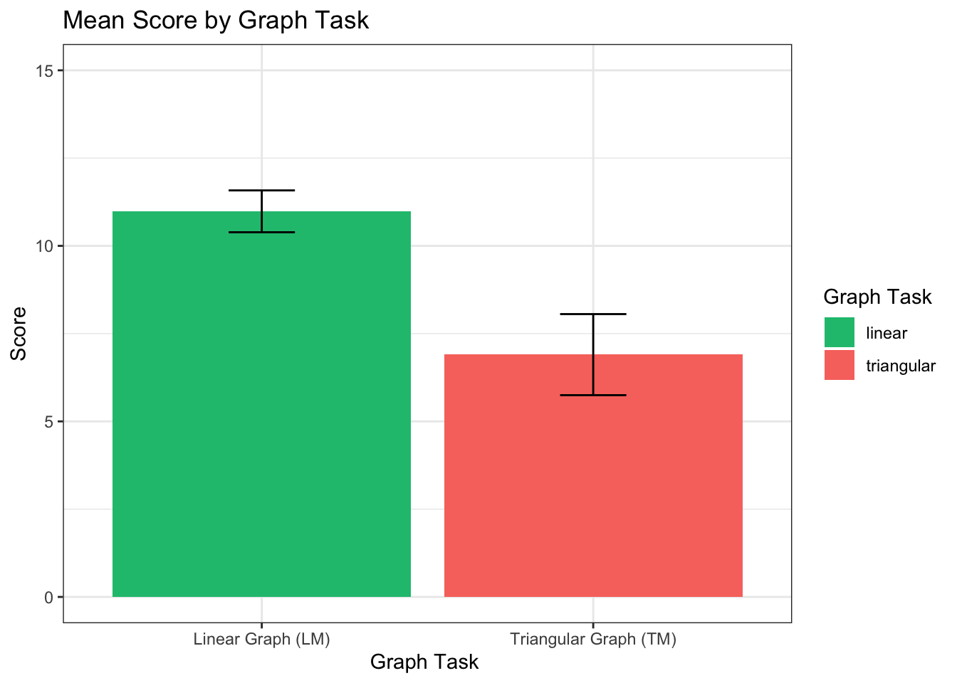
Hypothesis 3: Learners with (any form of) scaffolding will perform better with the TM than LM (replication of Qiang et al (2014)).
If we compare LM and TM scores in each scaffold condition (2-4) we expect to find that TM scores are higher than LM scores. Instead, we find that TM scores are on average lower than LM scores in every condition.
#explore descriptive statistics based on each IV
desc <- by(df_subjects2$score_diff, list(df_subjects2$condition), stat.desc, basic=FALSE)
desc
## : 0
##       median         mean      SE.mean CI.mean.0.95          var      std.dev
##   -4.0000000   -4.0819672    0.5774899    1.1551518   20.3431694    4.5103403
##     coef.var
##   -1.1049428
## ------------------------------------------------------------
## : 1
##       median         mean      SE.mean CI.mean.0.95          var      std.dev
##    -2.000000    -2.254237     0.511466     1.023810    15.434249     3.928645
##     coef.var
##    -1.742782
## ------------------------------------------------------------
## : 2
##       median         mean      SE.mean CI.mean.0.95          var      std.dev
##   -2.0000000   -2.1969697    0.4943597    0.9873044   16.1298368    4.0161968
##     coef.var
##   -1.8280620
## ------------------------------------------------------------
## : 3
##       median         mean      SE.mean CI.mean.0.95          var      std.dev
##   -1.0000000   -2.3548387    0.5085711    1.0169507   16.0359598    4.0044925
##     coef.var
##   -1.7005379
## ------------------------------------------------------------
## : 4
##       median         mean      SE.mean CI.mean.0.95          var      std.dev
##    0.5000000   -0.2205882    0.3913269    0.7810919   10.4133011    3.2269647
##     coef.var
##  -14.6289066
# LM_mean = desc_control$linear_score[2]
# LM_SD = desc_control$linear_score[6]
# TM_mean = desc_control$triangular_score[2]
# TM_SD = desc_control$triangular_score[6]
bar <- ggplot(df_subjects2, aes(x = condition, y= score_diff))
bar + stat_summary(aes(y = score_diff, group=condition), fun.y=mean, geom="bar", position="dodge") +
stat_summary(fun.data = mean_cl_normal, geom="errorbar", position = position_dodge(width=0.9),width=0.2) +
labs (x = "Scaffold", y= "Score Difference (TM-LM)") +
coord_cartesian(ylim=c(-15,15)) +
theme_bw() +
theme(strip.background = element_blank()) +
ggtitle("Score Difference by Scaffold") +
scale_x_discrete(labels=c( "0" = "none-control", "1" = "what-text", "2"="how-text", "3"="static-img", "4"="ix img")) 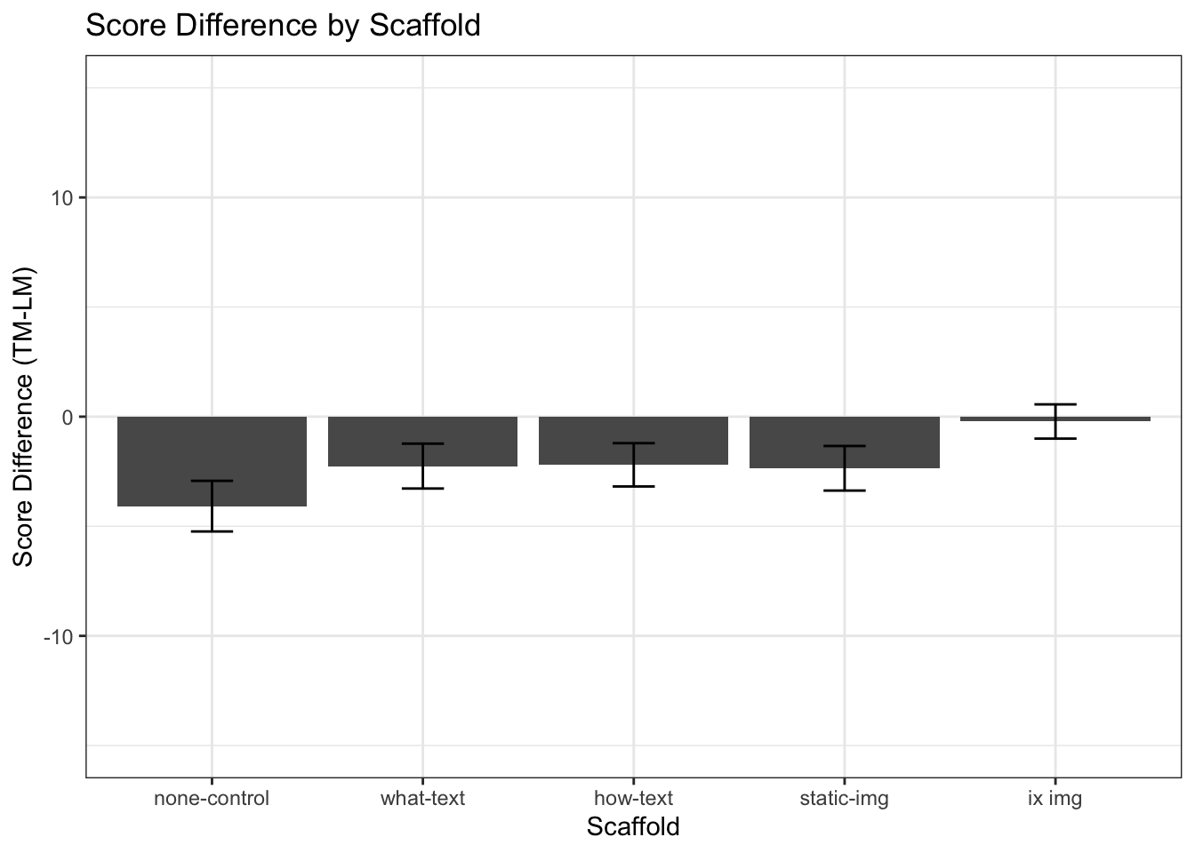
#REPEATED MEASURES ANOVA ON score by scaffold condition

#One way to look at this is an ANOVA on the difference score by scaffold condition
#construct contrasts for ANOVA model
options(contrasts=c("contr.sum","contr.poly"))

simpleModel = ezANOVA(data = df_subjects2,
                     dv = .(score_diff),
                     wid = .(subject),
                     between = .(condition),
                     type = 3,
                     detailed = TRUE)
## Warning: Converting "subject" to factor for ANOVA.
## Warning: Data is unbalanced (unequal N per group). Make sure you specified a
## well-considered value for the type argument to ezANOVA().
## Coefficient covariances computed by hccm()
simpleModel
## $ANOVA
##        Effect DFn DFd       SSn      SSd        F            p p<.05        ges
## 1 (Intercept)   1 311 1555.5595 4840.101 99.95226 1.373019e-20     * 0.24322110
## 2   condition   4 311  483.9752 4840.101  7.77444 5.544654e-06     * 0.09090314
##
## $`Levene's Test for Homogeneity of Variance`
##   DFn DFd      SSn      SSd        F          p p<.05
## 1   4 311 65.26842 1928.592 2.631256 0.03443319     *


pairwise.t.test(df_subjects2$score_diff, df_subjects2$condition,  p.adjust.method="bonferroni")
##
##  Pairwise comparisons using t tests with pooled SD
##
## data:  df_subjects2$score_diff and df_subjects2$condition
##
##   0       1     2     3
## 1 0.117   -     -     -
## 2 0.075   1.000 -     -
## 3 0.158   1.000 1.000 -
## 4 6.1e-07 0.040 0.040 0.022
##
## P value adjustment method: bonferroni
Instead, we find that only in the interactive-image condition yields TM scores significantly higher than the no-scaffold control.
###MIXED EFFECTS MODEL
Compute mixed effects ANOVA on Response Score
Significant main effect of Graph F(1,297) = 97.67, p < .001
Significant main effect of Scaffold F(4,297) = 4.24, p < .01
Significant main effect of Scenario F(1,297) = 22.29, p < .001
Significant interaction of Scaffold and Graph F(4,297) = 9.99, p
<.001
Significant interaction of Graph and Scenario F(1,297) = 34.80, p
<.001
#construct contrasts for ANOVA model
options(contrasts=c("contr.sum","contr.poly"))

#execute the model
mixedModel = ezANOVA(data = l_scores,
                     dv = .(value),
                     wid = .(subject),
                     between = .(condition,order,lm_scenarios),
                     within = .(variable),
                     type = 3,
                     detailed = TRUE)
## Warning: Converting "subject" to factor for ANOVA.## Warning: Data is unbalanced (unequal N per group). Make sure you specified a
## well-considered value for the type argument to ezANOVA().mixedModel## $ANOVA
## Effect DFn DFd SSn SSd
## 1 (Intercept) 1 296 6.032444e+04 4314.409
## 2 condition 4 296 2.474212e+02 4314.409
## 3 order 1 296 1.070270e+01 4314.409
## 4 lm_scenarios 1 296 3.243464e+02 4314.409
## 9 variable 1 296 6.708253e+02 2053.170
## 5 condition:order 4 296 3.979850e+01 4314.409
## 6 condition:lm_scenarios 4 296 7.450472e+01 4314.409
## 7 order:lm_scenarios 1 296 6.306627e-01 4314.409
## 10 condition:variable 4 296 2.785593e+02 2053.170
## 11 order:variable 1 296 2.378837e+01 2053.170
## 12 lm_scenarios:variable 1 296 2.382161e+02 2053.170
## 8 condition:order:lm_scenarios 4 296 2.393475e+01 4314.409
## 13 condition:order:variable 4 296 5.603432e+01 2053.170
## 14 condition:lm_scenarios:variable 4 296 2.757067e+01 2053.170
## 15 order:lm_scenarios:variable 1 296 1.699674e+00 2053.170
## 16 condition:order:lm_scenarios:variable 4 296 8.360845e+00 2053.170
## F p p<.05 ges
## 1 4.138698e+03 4.967248e-176 * 9.045226e-01
## 2 4.243727e+00 2.351329e-03 * 3.740306e-02
## 3 7.342835e-01 3.921915e-01 1.677991e-03
## 4 2.225254e+01 3.689436e-06 * 4.846832e-02
## 9 9.671109e+01 6.226124e-20 * 9.530930e-02
## 5 6.826171e-01 6.044789e-01 6.211356e-03
## 6 1.277892e+00 2.786863e-01 1.156531e-02
## 7 4.326807e-02 8.353644e-01 9.903297e-05
## 10 1.003979e+01 1.241419e-07 * 4.191296e-02
## 11 3.429505e+00 6.503691e-02 3.721953e-03
## 12 3.434297e+01 1.230461e-08 * 3.606168e-02
## 8 4.105247e-01 8.010291e-01 3.744770e-03
## 13 2.019580e+00 9.169296e-02 8.723179e-03
## 14 9.936975e-01 4.112221e-01 4.311185e-03
## 15 2.450374e-01 6.209585e-01 2.668550e-04
## 16 3.013402e-01 8.769499e-01 1.311312e-03#summary(mixedModel)####MAIN EFFECT: Graph on SCORE
On average, participants scored significantly higher on the linear model
task (M = 10.96, SD = 2.13) than on the triangular model (M = 8.78 SD =
4.44), t(316) = 9.41, p < 0.001, r = 0.47
bar <- ggplot(l_scores, aes(x = variable, y= value, fill=variable))
bar + stat_summary(aes(y = value, group=variable), fun.y=mean,  geom="bar", position="dodge") +
      stat_summary(fun.data = mean_cl_normal, geom="errorbar", position = position_dodge(width=0.9),width=0.2) +
      labs (x = "Graph Task ", y= "Score", fill="Graph Task") +
      coord_cartesian(ylim=c(0,15)) +
      scale_x_discrete(labels=c("linear_score" = "Linear Graph (LM)", "triangular_score" = "Triangular Graph (TM)")) +
      theme_bw() +
      theme(strip.background = element_blank()) +
      ggtitle("Mean Score by Graph Task")+
      scale_fill_manual(values = c(green,red),
                        name = "Graph Task",
                        breaks =c("linear_score", "triangular_score"),
                        labels =c("linear","triangular"))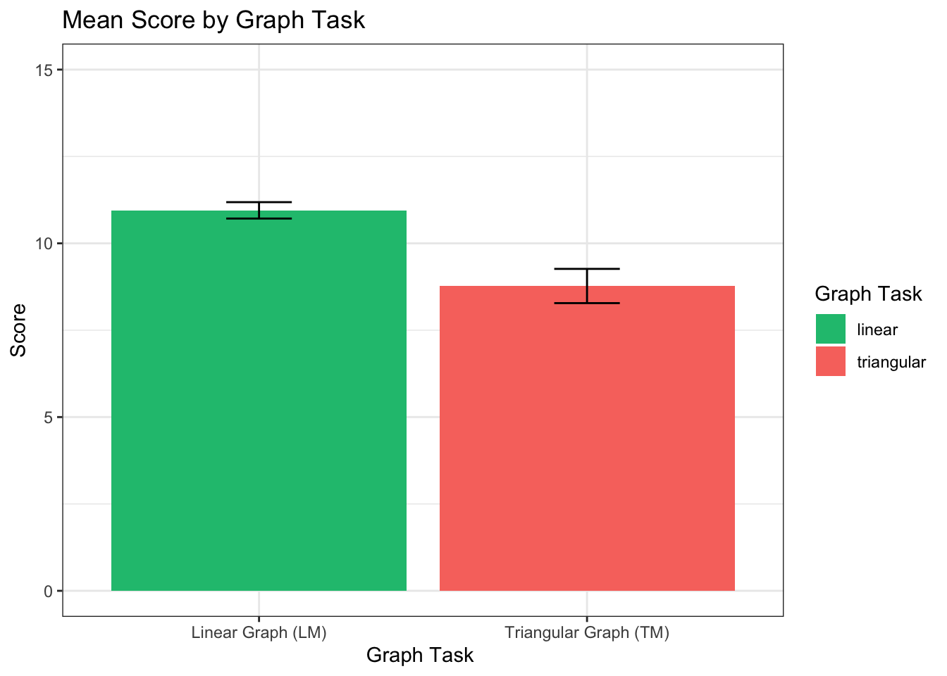
#CALULCULATE POSTHOC DIFFERENCE & EFFECT SIZE
mainEffectGraph  <- t.test(value ~ variable, data=l_scores, paired=TRUE)
mainEffectGraph
##
## Paired t-test
##
## data: value by variable
## t = 9.4141, df = 315, p-value < 2.2e-16
## alternative hypothesis: true mean difference is not equal to 0
## 95 percent confidence interval:
## 1.722182 2.632249
## sample estimates:
## mean difference
## 2.177215t <-mainEffectGraph$statistic[[1]]
df <-mainEffectGraph$parameter[[1]]
r <- sqrt(t^2/(t^2+df))
round(r,3)## [1] 0.469####MAIN EFFECT: Scaffold on SCORE ####MAIN EFFECT: Scenario on SCORE
When answering questions (with either graph) in the axis scenario (M = 9.20, SD = 4.12), participants had significantly lower scores, t(316) = -4.77, p < 0.001, r = -.26, than in the longmire scenario (M = 10.52, SD = 2.97)
#RUN ANCOVA ON tm_score with lm_score as covariate
# model.1=aov(triangular_score~linear_score+condition, data=df_subjects2)
#
# Anova(model.1, type="III")
#ANCOVA PRECONDITIONS
#1. linear relationship between covariate and dependent variable
#2. all treatment (condition) regression lines have same slope
test<-lm(formula = triangular_score ~ linear_score + condition, data = df_subjects2)
summary(test)
##
## Call:
## lm(formula = triangular_score ~ linear_score + condition, data = df_subjects2)
##
## Residuals:
## Min 1Q Median 3Q Max
## -11.4165 -2.4270 0.5835 2.7139 8.3945
##
## Coefficients:
## Estimate Std. Error t value Pr(>|t|)
## (Intercept) -0.33157 1.16079 -0.286 0.775
## linear_score 0.82742 0.10404 7.953 3.43e-14 ***
## condition1 -1.85485 0.44871 -4.134 4.60e-05 ***
## condition2 -0.01259 0.45457 -0.028 0.978
## condition3 0.01467 0.43570 0.034 0.973
## condition4 -0.13881 0.44597 -0.311 0.756
## ---
## Signif. codes: 0 '***' 0.001 '**' 0.01 '*' 0.05 '.' 0.1 ' ' 1
##
## Residual standard error: 3.934 on 310 degrees of freedom
## Multiple R-squared: 0.2311, Adjusted R-squared: 0.2187
## F-statistic: 18.64 on 5 and 310 DF, p-value: 3.427e-16bar <- ggplot(l_scores, aes(x = variable, y= value, fill=lm_scenarios))
bar + stat_summary(aes(y = value, group=lm_scenarios), fun.y=mean, geom="bar", position="dodge") +
stat_summary(fun.data = mean_cl_normal, geom="errorbar", position = position_dodge(width=0.9),width=0.2) +
labs (x = "Graph Task", y= "Score", fill="") +
coord_cartesian(ylim=c(0,15)) +
scale_x_discrete(labels=c("linear_score" = "linear (LM)", "triangular_score" = "triangular (TM)")) +
theme_bw() +
theme(strip.background = element_blank()) +
ggtitle("Mean Score by Scenario & Graph")+
scale_fill_manual(values = c(blue,purple),
name = "Task Scenario",
breaks =c("axis","longmire"),
labels =c("axis","longmire"))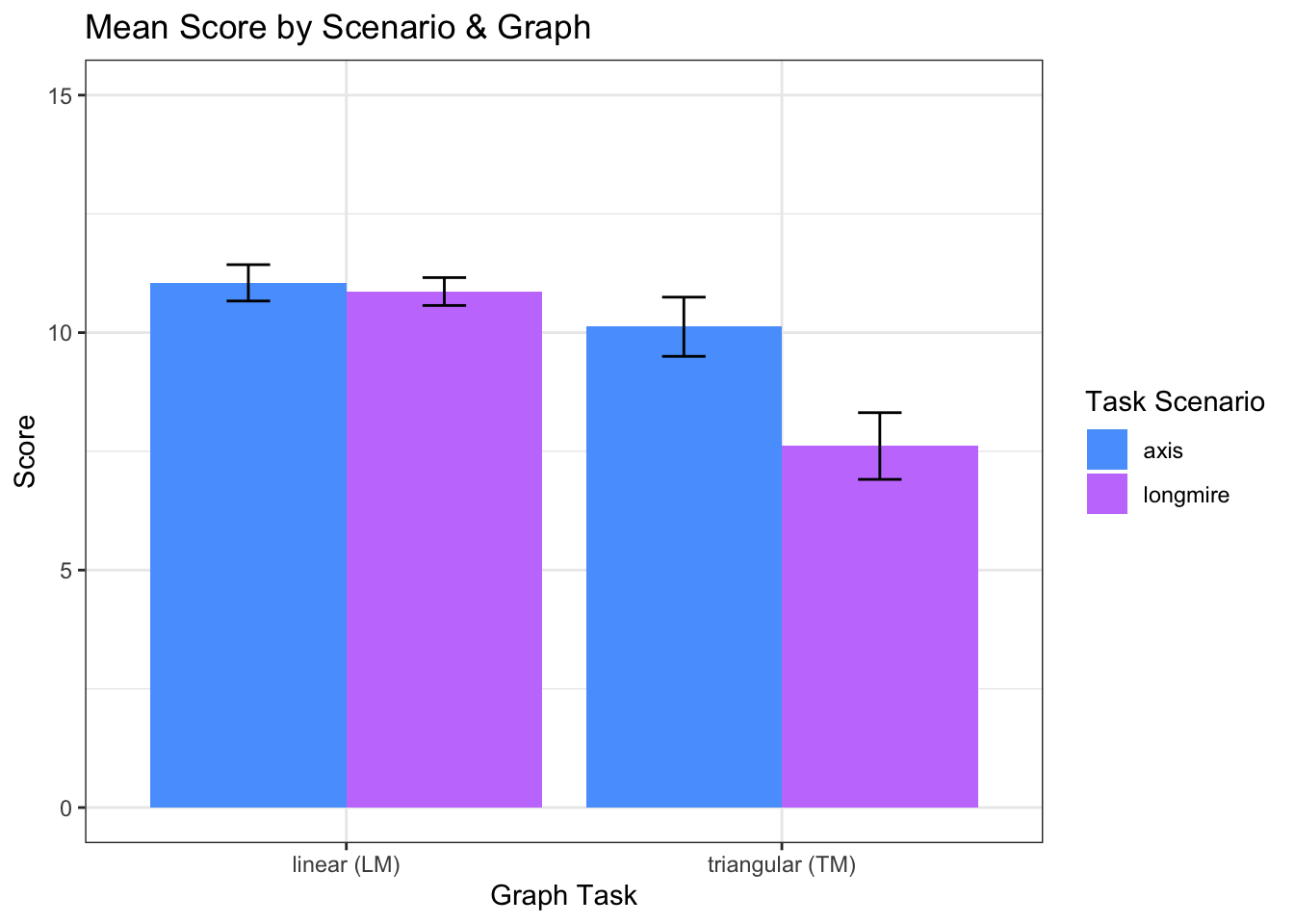
dots <- ggplot(l_scores, aes(x = lm_scenarios, y= value, color=variable))
dots + stat_summary(aes(y = value, group=variable), fun.y=mean, geom="point", position = position_dodge(width=0.1),width=0.2) +
stat_summary(fun.data = mean_cl_normal, geom="errorbar", position = position_dodge(width=0.1),width=0.2) +
stat_summary(aes(y = value, group=variable), fun.y=mean, geom="line", position=position_dodge(width=0.1)) +
labs (x = "Task Scenario ", y= "Score", fill="Task Graph") +
coord_cartesian(ylim=c(0,15)) +
scale_x_discrete(labels=c("axis" = "axis", "longmire" = "longmire")) +
theme_bw() +
theme(strip.background = element_blank()) +
ggtitle("Mean Score by Scenario & Graph")+
scale_color_manual(values = c(green,red),
name = "Task Graph",
breaks =c("linear_score", "triangular_score"),
labels =c("linear (LM)","triangular (TM)"))## Warning in stat_summary(aes(y = value, group = variable), fun.y = mean, :
## Ignoring unknown parameters: `width`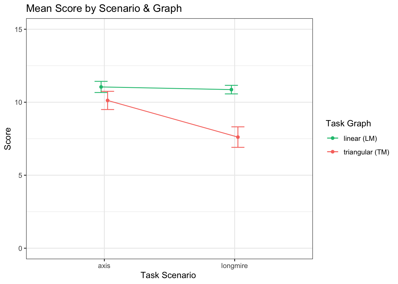
####INTERACTION: Scaffold & Graph
####INTERACTION: Scenario & Graph
Results (Time)
####Explore the data We see comparable response times for LM and TM graphs when the LM graph is solved first. However, when the TM graph is solved first, the TM graph-reading task seems to take much longer.
#EXPLORE THE DATA
#SIMPLE BOXPLOT BY CONDITION
# mixedPlot_condition <- ggplot(l_times, aes(condition,value, color=variable))+ geom_boxplot() +
# labs(x="scaffold condition", y="time (mins)") +
# ggtitle("Response Time by Scaffold ") +
# theme_bw()
# mixedPlot_condition
#BOXPLOT BY CONDITION, FACET WITH ORDER
mixedPlot_order <- ggplot(l_times, aes(condition,value, fill=variable))+ geom_boxplot() +
facet_wrap(~order, labeller=labeller(order = order_labels)) +
labs(x="scaffold condition", y="time (mins)", color="task")+
labs(title="Response Time by Scaffold & Graph-Order ") +
theme_bw() +
theme(strip.background = element_blank()) +
scale_fill_manual( values = c(green,red),
name="graphing task",
breaks=c("LM_T_M", "TM_T_M"),
labels=c("linear", "triangular"))
mixedPlot_order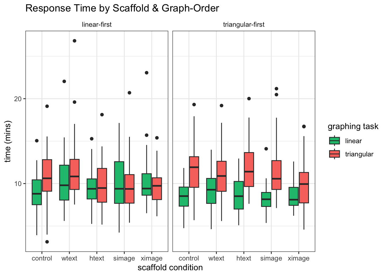
#BOXPLOT BY CONDITION, FACET WITH ORDER AND SCENARIO
mixedPlot_scenario <- ggplot(l_times, aes(condition,value, fill=variable))+ geom_boxplot() +
facet_grid(lm_scenarios~order, labeller=labeller(order = order_labels)) +
labs(x="scaffold condition", y="time (mins)")+
ggtitle("Response Time by Scaffold, Task Order and Scenario ") +
theme_bw() +
theme(strip.background = element_blank()) +
scale_fill_manual( values = c(green,red),
name="graphing task",
breaks=c("LM_T_M", "TM_T_M"),
labels=c("linear", "triangular"))
mixedPlot_scenario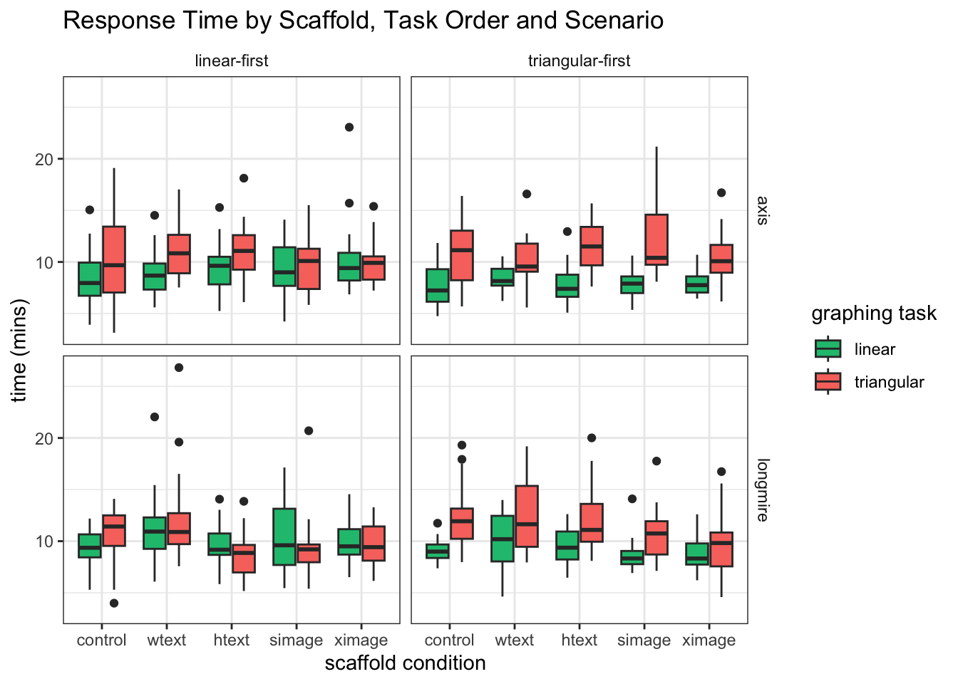
####Hypothesis Testing
Compute mixed effects ANOVA on Response Time
Significant main-effect of Graph F(1,297) = 109.71, p <.001
Significant interaction between Graph & Scaffold F(4,297) = 3.51, p
< .01
Significant interaction between Graph and Scenario, F(1,297) = 8.35, p
<.01
Significant interaction between Graph and Graph-Order, F(1,297) = 44.24,
p <.001
#construct contrasts for ANOVA model
options(contrasts=c("contr.sum","contr.poly"))
#execute the model
mixedModel = ezANOVA(data = l_times,
dv = .(value),
wid = .(subject),
between = .(condition,order,lm_scenarios),
within = .(variable),
type = 3,
detailed = TRUE)## Warning: Converting "subject" to factor for ANOVA.## Warning: Data is unbalanced (unequal N per group). Make sure you specified a
## well-considered value for the type argument to ezANOVA().mixedModel## $ANOVA
## Effect DFn DFd SSn SSd
## 1 (Intercept) 1 296 6.152673e+04 3625.023
## 2 condition 4 296 5.451453e+01 3625.023
## 3 order 1 296 5.412868e-01 3625.023
## 4 lm_scenarios 1 296 3.302950e+01 3625.023
## 9 variable 1 296 4.245147e+02 1145.391
## 5 condition:order 4 296 3.644702e+01 3625.023
## 6 condition:lm_scenarios 4 296 8.098356e+01 3625.023
## 7 order:lm_scenarios 1 296 1.703814e+01 3625.023
## 10 condition:variable 4 296 5.436523e+01 1145.391
## 11 order:variable 1 296 1.711826e+02 1145.391
## 12 lm_scenarios:variable 1 296 3.232806e+01 1145.391
## 8 condition:order:lm_scenarios 4 296 3.690296e+01 3625.023
## 13 condition:order:variable 4 296 3.440708e+01 1145.391
## 14 condition:lm_scenarios:variable 4 296 2.334054e+01 1145.391
## 15 order:lm_scenarios:variable 1 296 2.473067e-01 1145.391
## 16 condition:order:lm_scenarios:variable 4 296 2.271490e+01 1145.391
## F p p<.05 ges
## 1 5.023944e+03 9.890040e-188 * 9.280450e-01
## 2 1.112841e+00 3.505529e-01 1.129852e-02
## 3 4.419859e-02 8.336292e-01 1.134546e-04
## 4 2.697013e+00 1.015984e-01 6.876213e-03
## 9 1.097060e+02 4.807775e-22 * 8.171713e-02
## 5 7.440173e-01 5.626588e-01 7.582291e-03
## 6 1.653171e+00 1.609305e-01 1.669283e-02
## 7 1.391244e+00 2.391423e-01 3.558916e-03
## 10 3.512361e+00 8.058308e-03 * 1.126792e-02
## 11 4.423822e+01 1.402607e-10 * 3.464116e-02
## 12 8.354442e+00 4.132080e-03 * 6.731167e-03
## 8 7.533247e-01 5.564595e-01 7.676416e-03
## 13 2.222929e+00 6.656133e-02 7.160949e-03
## 14 1.507956e+00 1.997993e-01 4.868948e-03
## 15 6.391074e-02 8.005938e-01 5.183909e-05
## 16 1.467536e+00 2.120297e-01 4.739055e-03#summary(mixedModel)####MAIN EFFECT: Graph on TIME
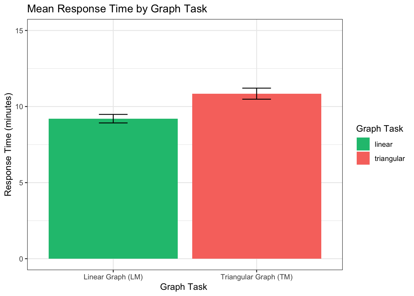
On average, participants spent significantly more time on triangular
model task (M = 10.84, SD = 3.28) than on the linear model (M = 9.20, SD
= 2.53), t(316) = -9.46, p < 0.001, r = 0.47
##
## Paired t-test
##
## data: value by variable
## t = -9.458, df = 315, p-value < 2.2e-16
## alternative hypothesis: true mean difference is not equal to 0
## 95 percent confidence interval:
## -1.984566 -1.301067
## sample estimates:
## mean difference
## -1.642816## [1] 0.47####INTERACTION: Scaffold & Graph
####INTERACTION: Scenario & Graph
####INTERACTION: Order & Graph
Results (Graph Drawing)
# #explore independence of graph drawing by condition
# table(df_subjects2$`Graph Type`, df_subjects2$condition)
# chisq.test(df_subjects2$`Graph Type`, df_subjects2$condition, correct=TRUE)
# fisher.test(df_subjects2$`Graph Type`, df_subjects2$condition)
#
# Input =("
# Interpretation control whattext howtext static interactive
# 'Right angle' 17 6 9 10 2
# 'Triangular' 34 50 48 41 57
# 'Linear' 6 0 3 7 1
# 'Scatterplot' 0 0 0 0 0
# 'Asymmetric' 3 3 5 4 7
# ")
#
# Matriz = as.matrix(read.table(textConnection(Input),
# header=TRUE,
# row.names=1))
#
# Matriz
#
# chisq.test(Matriz)
#
# pairwiseNominalIndependence(Matriz,
# fisher = FALSE,
# gtest = FALSE,
# chisq = TRUE,
# method = "fdr")
#
#
# FUN = function(i,j){
# chisq.test(matrix(c(Matriz[i,1], Matriz[i,2],
# Matriz[j,1], Matriz[j,2]),
# nrow=2,
# byrow=TRUE))$ p.value
# }
#
# pairwise.table(FUN,
# rownames(Matriz),
# p.adjust.method="none")
#explore independence of graph drawing by order
table(df_subjects2$`Graph Type`, df_subjects2$order)
##
## LMFirst TMFirst
## Triangular (right angle) 21 23
## Triangular 122 108
## Linear Model 3 14
## Scatterplot 0 3
## Other 0 0
## Triangular (asymmetric) 8 14
chisq.test(df_subjects2$`Graph Type`, df_subjects2$order, correct=TRUE)
## Warning in chisq.test(df_subjects2$`Graph Type`, df_subjects2$order, correct =
## TRUE): Chi-squared approximation may be incorrect
##
## Pearson's Chi-squared test
##
## data: df_subjects2$`Graph Type` and df_subjects2$order
## X-squared = 12.503, df = 4, p-value = 0.01398
fisher.test(df_subjects2$`Graph Type`, df_subjects2$order)
##
## Fisher's Exact Test for Count Data
##
## data: df_subjects2$`Graph Type` and df_subjects2$order
## p-value = 0.01117
## alternative hypothesis: two.sided
# ftable(bigTable)The cell sizes are too heterogeneous to look for correlations in TM score and drawing type, but we can directly compare the TM scores for the two triangular interpretations: the right-angle triangle and asymetric triangle.
#SETUP DATA FOR RESPONSE ACCURACY ANALYSIS
df_small_draw <- subset(df_subjects2, df_subjects2$`Graph Type`%in% c("Triangular (asymmetric)","Triangular (right angle)"))
#LM SCORES BY SCAFFOLD
desc_control <- by(df_small_draw$triangular_score, df_small_draw$`Graph Type`, stat.desc, basic=FALSE)
desc_control
## df_small_draw$`Graph Type`: Triangular (right angle)
## median mean SE.mean CI.mean.0.95 var std.dev
## 2.0000000 2.2954545 0.2990110 0.6030131 3.9339323 1.9834143
## coef.var
## 0.8640617
## ------------------------------------------------------------
## df_small_draw$`Graph Type`: Triangular
## NULL
## ------------------------------------------------------------
## df_small_draw$`Graph Type`: Linear Model
## NULL
## ------------------------------------------------------------
## df_small_draw$`Graph Type`: Scatterplot
## NULL
## ------------------------------------------------------------
## df_small_draw$`Graph Type`: Other
## NULL
## ------------------------------------------------------------
## df_small_draw$`Graph Type`: Triangular (asymmetric)
## median mean SE.mean CI.mean.0.95 var std.dev
## 9.0000000 8.5454545 0.7942632 1.6517607 13.8787879 3.7254245
## coef.var
## 0.4359539
right_mean = desc_control$`Triangular (right angle)`[2]
right_SD = desc_control$`Triangular (right angle)`[6]
asy_mean = desc_control$`Triangular (asymmetric)`[2]
asy_SD = desc_control$`Triangular (asymmetric)`[6]
# #CALULCULATE POSTHOC DIFFERENCE & EFFECT SIZE
mainEffectGraph <- t.test(triangular_score ~ `Graph Type`, data=df_small_draw, na.rm=TRUE)
mainEffectGraph
##
## Welch Two Sample t-test
##
## data: triangular_score by Graph Type
## t = -7.3644, df = 27.108, p-value = 6.223e-08
## alternative hypothesis: true difference in means between group Triangular (right angle) and group Triangular (asymmetric) is not equal to 0
## 95 percent confidence interval:
## -7.991027 -4.508973
## sample estimates:
## mean in group Triangular (right angle) mean in group Triangular (asymmetric)
## 2.295455 8.545455
t <-mainEffectGraph$statistic[[1]]
df <-mainEffectGraph$parameter[[1]]
r <- sqrt(t^2/(t^2+df))
round(r,3)
## [1] 0.817TM scores for participants who drew “right-angle” graphs were significantly lower (M = 2.3, SD = 1.98) than for participants who drew “asymmetric triangle” graphs (M = 8.55, SD = 3.73), t(27.1083223) = -7.3643582, p = 1.9116967^{-9} , r = 0.8165396.
See GALLERY of all images hereReferences
Qiang, Y., Valcke, M., De Maeyer, P., & Van de Weghe, N. (2014). Representing time intervals in a two-dimensional space: An empirical study. Journal of Visual Languages and Computing, 25(4), 466–480.
Power Analyses
In order to estimate the number of subjects needed for future study, we will evaluate the statistical significance and effect size of any differences in accuracy scores between scaffold groups for the TM-graph only, in the TM-first graph order.
#explore descriptive statistics based on each IV
desc <- by(df_subjects2$triangular_score, list(df_subjects2$condition), stat.desc, basic=FALSE)
desc
## : 0
##       median         mean      SE.mean CI.mean.0.95          var      std.dev
##    6.0000000    6.9016393    0.5772106    1.1545931   20.3234973    4.5081590
##     coef.var
##    0.6532012
## ------------------------------------------------------------
## : 1
##       median         mean      SE.mean CI.mean.0.95          var      std.dev
##   10.0000000    8.8135593    0.5568103    1.1145770   18.2922268    4.2769413
##     coef.var
##    0.4852683
## ------------------------------------------------------------
## : 2
##       median         mean      SE.mean CI.mean.0.95          var      std.dev
##   10.0000000    8.6969697    0.5801574    1.1586543   22.2144522    4.7132210
##     coef.var
##    0.5419383
## ------------------------------------------------------------
## : 3
##       median         mean      SE.mean CI.mean.0.95          var      std.dev
##   10.0000000    8.5645161    0.5806782    1.1611378   20.9056055    4.5722648
##     coef.var
##    0.5338614
## ------------------------------------------------------------
## : 4
##       median         mean      SE.mean CI.mean.0.95          var      std.dev
##   11.0000000   10.6764706    0.4129389    0.8242294   11.5952590    3.4051812
##     coef.var
##    0.3189426
# LM_mean = desc_control$linear_score[2]
# LM_SD = desc_control$linear_score[6]
# TM_mean = desc_control$triangular_score[2]
# TM_SD = desc_control$triangular_score[6]
bar <- ggplot(df_subjects2, aes(x = condition, y= triangular_score))
bar + stat_summary(aes(y = triangular_score, group=condition), fun.y=mean, geom="bar", position="dodge") +
stat_summary(fun.data = mean_cl_normal, geom="errorbar", position = position_dodge(width=0.9),width=0.2) +
labs (x = "Scaffold", y= "Score Difference (TM-LM)") +
coord_cartesian(ylim=c(0,15)) +
theme_bw() +
theme(strip.background = element_blank()) +
ggtitle("TM Score by Scaffold for TM-first Order ") +
scale_x_discrete(labels=c( "0" = "none-control", "1" = "what-text", "2"="how-text", "3"="static-img", "4"="ix img")) 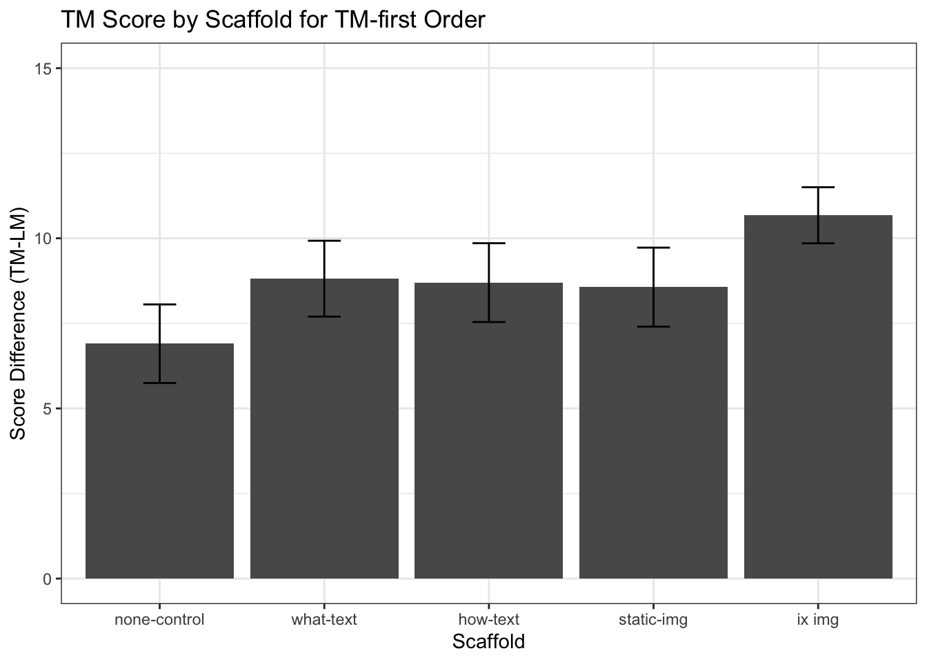
#ONE WAY ANOVA ON triangular score BY SCAFFOLD
#construct contrasts for ANOVA model
options(contrasts=c("contr.sum","contr.poly"))

simpleModel = ezANOVA(data = w_scores,
                     dv = .(triangular_score),
                     wid = .(subject),
                     between = .(condition),
                     type = 3,
                    detailed = TRUE)
## Warning: Converting "subject" to factor for ANOVA.## Warning: Data is unbalanced (unequal N per group). Make sure you specified a
## well-considered value for the type argument to ezANOVA().## Coefficient covariances computed by hccm()simpleModel$ANOVA## Effect DFn DFd SSn SSd F p p<.05
## 1 (Intercept) 1 311 24021.4468 5776.423 1293.303895 8.013810e-113 *
## 2 condition 4 311 463.1723 5776.423 6.234247 7.754407e-05 *
## ges
## 1 0.80614645
## 2 0.07423114the GES is the (generalized eta squared)
Eta-square (η2) is an effect size measurement for the analysis of variance (ANOVA). It measures the strength of the effect on a continuous field. The effect can be the main effect of one field or the interaction effect of two fields. Eta-square can be interpreted as the proportion of variance in the continuous target field explained by an effect while controlling for other effects. It is calculated by dividing the sum of squares for the effect by the total sum of squares. Table 1. Interpretation of effect size when there is one input (One-way ANOVA) Effect size (ES) Interpretation ES ≤ 0.04 The effect is statistically significant but weak. 0.04 < ES ≤ 0.36 The effect is moderate. ES > 0.36 The effect is strong.
Copyright © 2018 Amy Rae Fox. All rights reserved.